Features of HANA (Hybrid In-Memory Database):
No Disk

In-Memory Computing
 High performance
in-memory computing will change how enterprises work. Currently, enterprise
data is split into two databases for performance reasons. Disk-based
row-oriented database systems are used for operational data (e.g. "insert
or update a specific sales order") and column-oriented databases are used
for analytics (e.g. “sum of all sales in China grouped by product”). While
analytical databases are often kept in-memory, they can also be mixed with
disk-based storage media.
High performance
in-memory computing will change how enterprises work. Currently, enterprise
data is split into two databases for performance reasons. Disk-based
row-oriented database systems are used for operational data (e.g. "insert
or update a specific sales order") and column-oriented databases are used
for analytics (e.g. “sum of all sales in China grouped by product”). While
analytical databases are often kept in-memory, they can also be mixed with
disk-based storage media.
Read more at http://www.no-disk.com/
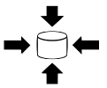
Active and Passive Data Store
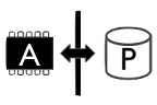 By default, all data is
stored in-memory to achieve high-speed data access. However, not all data is
accessed or updated frequently and needs to reside in-memory, as this increases
the required amount of main memory unnecessarily. This so-called historic or
passive data can be stored in a specific passive data storage based on less
expensive storage media, such as SSDs or hard disks, still providing sufficient
performance for possible accesses at lower cost. The dynamic transition from
active to passive data is supported by the database, based on custom rules
defined as per customer needs.
By default, all data is
stored in-memory to achieve high-speed data access. However, not all data is
accessed or updated frequently and needs to reside in-memory, as this increases
the required amount of main memory unnecessarily. This so-called historic or
passive data can be stored in a specific passive data storage based on less
expensive storage media, such as SSDs or hard disks, still providing sufficient
performance for possible accesses at lower cost. The dynamic transition from
active to passive data is supported by the database, based on custom rules
defined as per customer needs.
We define two categories of data stores:
active and passive: We refer to active data when it is accessed frequently and
updates are expected (e.g., access rules). In contrast, we refer to passive
data when this data either is not used frequently and neither updated nor read.
Passive data is purely used for analytical and statistical purposes or in
exceptional situations where specific investigations require this data. A possible storage hierarchy is given by memory registers,
cache memory, main memory, flash storages, solid state disks, SAS hard disk
drives, SATA hard disk drives, tapes, etc. As a result, rules for migrating
data from one store to another need to be defined, we refer to it as aging
strategy or aging rules. The process of aging data, i.e. migrating it from a
faster store to a slower one, is considered as background tasks, which occurs
on regularly basis, e.g. weekly or daily. Since this process involves
reorganization of the entire data set, it should be processed during times with
low data access, e.g. during nights or weekends.
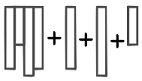
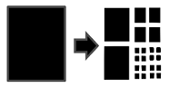
Combined Row and Column
Store
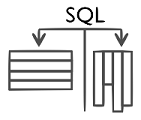 Column and row-oriented
storage in HANA provides the foundation to store data according to its frequent
usage patterns in column or in row-oriented manner to achieve optimal
performance. Through the usage of SQL, that supports column as well as
row-oriented storage, the applications on top stay oblivious to the choice of
storage layout.
Column and row-oriented
storage in HANA provides the foundation to store data according to its frequent
usage patterns in column or in row-oriented manner to achieve optimal
performance. Through the usage of SQL, that supports column as well as
row-oriented storage, the applications on top stay oblivious to the choice of
storage layout.
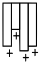
Minimal Projections
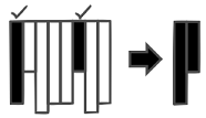 To increase the overall
performance, it is required to select only the minimal set of attributes that
should be projected for each query. This has two important advantages: First,
it dramatically reduces the amount of accessed data that is transferred between
client and server. Second, it reduces the number of accesses to random memory
locations and thus increases the overall performance
To increase the overall
performance, it is required to select only the minimal set of attributes that
should be projected for each query. This has two important advantages: First,
it dramatically reduces the amount of accessed data that is transferred between
client and server. Second, it reduces the number of accesses to random memory
locations and thus increases the overall performanceAny Attribute as an Index
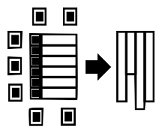 Traditional row-oriented
databases store tables as collections of tuples. To improve access to specific
values within columns and to avoid scanning the entire table, that is, all
columns and rows, indexes are typically created for these columns. The offsets of the matching
values are used as an index to retrieve the values of the remaining attributes,
avoiding the need to read data that is not required for the result set.
Consequently, complex objects can be filtered and retrieved via any of their
attributes.
Traditional row-oriented
databases store tables as collections of tuples. To improve access to specific
values within columns and to avoid scanning the entire table, that is, all
columns and rows, indexes are typically created for these columns. The offsets of the matching
values are used as an index to retrieve the values of the remaining attributes,
avoiding the need to read data that is not required for the result set.
Consequently, complex objects can be filtered and retrieved via any of their
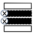
attributes.Insert-only
 Insert-only or append-only
describes how data is managed when inserting new data. The principle idea of
insert-only is that changes to existing data are handled by appending new
tuples to the data storage. Insert-only enables storing
the complete history of value changes and the latest value for a certain
attribute.For the history-based
access control, insert-only builds the basis to store the entire history of
queries for access decision. In addition, insert-only enables tracing of access
decision, which can be used to perform incident analysis
Insert-only or append-only
describes how data is managed when inserting new data. The principle idea of
insert-only is that changes to existing data are handled by appending new
tuples to the data storage. Insert-only enables storing
the complete history of value changes and the latest value for a certain
attribute.For the history-based
access control, insert-only builds the basis to store the entire history of
queries for access decision. In addition, insert-only enables tracing of access
decision, which can be used to perform incident analysis Group-Key
 A common access pattern of
enterprise applications is to select a small group of records from larger
relations. To speed up such queries,
group-key indexes can be defined that build on the compressed dictionary. A
group key index maps a dictionary-encoded value of a column to a list of
positions where this value can be found in a relation.
A common access pattern of
enterprise applications is to select a small group of records from larger
relations. To speed up such queries,
group-key indexes can be defined that build on the compressed dictionary. A
group key index maps a dictionary-encoded value of a column to a list of
positions where this value can be found in a relation. No Aggregate Tables

On-the-fly Extensibility
 The possibility of adding
new columns to existing database tables dramatically simplifies a wide range of
customization projects. In a column store database,
such as HANA, all columns are stored in physical separation from one another.
This allows for a simple implementation of column extensibility, which does not
need to update any other existing columns of the table. This reduces a schema
change to a pure metadata operation, allowing for flexible and real-time schema
extensions.
The possibility of adding
new columns to existing database tables dramatically simplifies a wide range of
customization projects. In a column store database,
such as HANA, all columns are stored in physical separation from one another.
This allows for a simple implementation of column extensibility, which does not
need to update any other existing columns of the table. This reduces a schema
change to a pure metadata operation, allowing for flexible and real-time schema
extensions. Reduction of Layers
 To avoid redundant data,
logical layers, describing the transformations, are executed during runtime,
thus increasing efficient use of hardware resources by removing all
materialized data maintenance task. Moving formalizable application logic to
the data it operates on results in a smaller application stack and increases
maintainability by code reduction. (Use Stored Procedures & other Business Fuction Libraries)
To avoid redundant data,
logical layers, describing the transformations, are executed during runtime,
thus increasing efficient use of hardware resources by removing all
materialized data maintenance task. Moving formalizable application logic to
the data it operates on results in a smaller application stack and increases
maintainability by code reduction. (Use Stored Procedures & other Business Fuction Libraries)
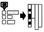
Partitioning
 We distinguish between two
partitioning approaches: vertical and horizontal partitioning, whereas a
combination of both approaches is also possible. Vertical partitioning refers
to the rearranging of individual database columns. It is achieved by splitting
columns of a database table into two or more column sets. Each of the column
sets can be distributed on individual databases servers. This can also be used
to build up database columns with different ordering to achieve better search
performance while guaranteeing high-availability of data. In contrast, horizontal
partitioning addresses large database tables and how to divide them into
smaller pieces of data. As a result, each piece of the database table contains
a subset of the complete data within the table. Splitting data into equivalent
long horizontal partitions is used to support search operations and better
scalability.
We distinguish between two
partitioning approaches: vertical and horizontal partitioning, whereas a
combination of both approaches is also possible. Vertical partitioning refers
to the rearranging of individual database columns. It is achieved by splitting
columns of a database table into two or more column sets. Each of the column
sets can be distributed on individual databases servers. This can also be used
to build up database columns with different ordering to achieve better search
performance while guaranteeing high-availability of data. In contrast, horizontal
partitioning addresses large database tables and how to divide them into
smaller pieces of data. As a result, each piece of the database table contains
a subset of the complete data within the table. Splitting data into equivalent
long horizontal partitions is used to support search operations and better
scalability.Lightweight Compression
 For in-memory databases, compression is
applied to reduce the amount of data that is transferred between main memory
and CPU, as well as to reduce overall main memory consumption. However, the
more complex the compression algorithm is, the more CPU cycles it will take to
decompress the data to perform query execution. As a result, in-memory
databases choose a trade-off between compression ration and performance using
so called light-weight compression algorithms.
For in-memory databases, compression is
applied to reduce the amount of data that is transferred between main memory
and CPU, as well as to reduce overall main memory consumption. However, the
more complex the compression algorithm is, the more CPU cycles it will take to
decompress the data to perform query execution. As a result, in-memory
databases choose a trade-off between compression ration and performance using
so called light-weight compression algorithms.Bulk Load
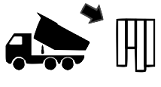 Besides transactional
inserts, HANA also supports a bulk load mode. This mode is designed to insert
large sets of data without the transactional overhead and thus enables
significant speed-ups when setting up systems or restoring previously collected
data.
Besides transactional
inserts, HANA also supports a bulk load mode. This mode is designed to insert
large sets of data without the transactional overhead and thus enables
significant speed-ups when setting up systems or restoring previously collected
data.Multi-core and Parallelization
 A CPU core can be considered as single worker
on a construction area. If it is possible to map each query to a single core,
the system’s response time is optimal. Query processing also involves data
processing, i.e. the database needs to be queried in parallel, too. If the
database is able to distribute the workload across multiple cores of a single
system, this is optimal. If the workload exceeds physical capacities of a
single system, multiple servers or blades need to be involved for work
distribution to achieve optimal processing behavior. From the database
perspective, the partitioning of data sets enables parallelization since
multiple cores across servers can be involved for data processing.
A CPU core can be considered as single worker
on a construction area. If it is possible to map each query to a single core,
the system’s response time is optimal. Query processing also involves data
processing, i.e. the database needs to be queried in parallel, too. If the
database is able to distribute the workload across multiple cores of a single
system, this is optimal. If the workload exceeds physical capacities of a
single system, multiple servers or blades need to be involved for work
distribution to achieve optimal processing behavior. From the database
perspective, the partitioning of data sets enables parallelization since
multiple cores across servers can be involved for data processing.
MapReduce
 MapReduce is a programming
model to parallelize the processing of large amounts of data. HANA emulates the MapReduce
programming model and allows the developer to define map functions as
user-defined procedures. Support for the MapReduce programming model enables
developers to implement specific analysis algorithms on HANA faster, without
worrying about parallelization and efficient execution by HANA’s calculation
engine.
MapReduce is a programming
model to parallelize the processing of large amounts of data. HANA emulates the MapReduce
programming model and allows the developer to define map functions as
user-defined procedures. Support for the MapReduce programming model enables
developers to implement specific analysis algorithms on HANA faster, without
worrying about parallelization and efficient execution by HANA’s calculation
engine.Dynamic Multithreading within Nodes

partitioning database tasks
on large data sets into as many jobs as threads are available on a given node.
This way, the maximal utilization of any supported hardware can be achieved.
Single and Multi-Tenancy
Analytics on Historical
Data
For analytics the historical data is the key. In HANA, historical data is
instantly available for analytical processing from solid state disk (SSD)
drives. Only active data is required to reside in-memory permanently.
Text Retrieval and
Exploration
Elements of search in unstructured data, such as linguistic or fuzzy search find their way into the domain of structured data, changing system interaction. Furthermore, for business environments added value lies in combining search in unstructured data with analytics of structured data.
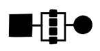
Object Data Guides
The in-memory database improves the retrieving performance of a business object by adding
 which is called object data guide and includes
two aspects: In addition to the parent instance, every node instance can
contain the link to the corresponding root instance. Using this additional
attribute, it is possible to retrieve all nodes in parallel instead of waiting
for the information from the parent level. Additionally, each node type in a
business object can be numbered. Then, for every root instance, a bit vector
(Object Data Guide) is stored, whose bit at position i indicates if an instance
of node number i exists for this root instance. Using this bit vector, a table
only needs to be checked if the corresponding bit is set, reducing the
complexity of queries to a minimum. This is mainly for Sparse tree data.
which is called object data guide and includes
two aspects: In addition to the parent instance, every node instance can
contain the link to the corresponding root instance. Using this additional
attribute, it is possible to retrieve all nodes in parallel instead of waiting
for the information from the parent level. Additionally, each node type in a
business object can be numbered. Then, for every root instance, a bit vector
(Object Data Guide) is stored, whose bit at position i indicates if an instance
of node number i exists for this root instance. Using this bit vector, a table
only needs to be checked if the corresponding bit is set, reducing the
complexity of queries to a minimum. This is mainly for Sparse tree data.

